Math 14 Preparing for Section 8.2: Applications of the Normal Distribution
TLDRThis video script discusses the application of the normal distribution in a study analyzing drive-through times at a fast-food restaurant. It explains how to calculate probabilities for various scenarios, such as the likelihood of a car spending less than 112 seconds, more than 175 seconds, and between two to three minutes in the drive-through. The script guides viewers through the process of finding z-scores, using normal distribution tables, and employing technology like StatCrunch and calculators to find areas under the curve. It also addresses the concept of unusual events by comparing the probability of a car spending over three minutes to the threshold of 0.05.
Takeaways
- 📚 The script discusses the application of the normal distribution in a specific scenario involving drive-through times at a fast food restaurant.
- ⏱ The mean drive-through time found in a study was 142.2 seconds with a standard deviation of 25 seconds.
- 🔍 The first task was to calculate the probability of a car getting through the drive-through in less than 112 seconds, which involved finding the z-score and using a standard normal distribution table.
- 📉 The z-score for the time of 112 seconds was calculated to be -1.21, indicating a value below the mean.
- 📊 Using the standard normal distribution table, the probability of a car taking less than 112 seconds was found to be approximately 0.1131.
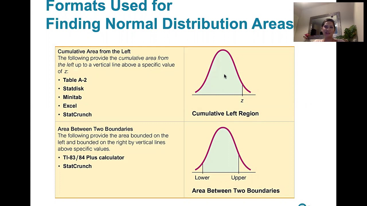
- 🛑 The script also covered how to use technology like StatCrunch and a calculator to find probabilities, offering an alternative to manual calculations.
- 🚗 For the second task, the probability of a car spending more than 175 seconds in the drive-through was calculated, resulting in a z-score of 1.31 and a probability of 0.0951.
- 📈 The third task involved finding the proportion of cars spending between two and three minutes (120 to 180 seconds) in the drive-through, which was found to be 0.7478.
- 🤔 The final question asked whether it would be unusual for a car to spend more than three minutes in the drive-through, with the probability calculated to be 0.0655.
- 📝 The script emphasized that an event is considered unusual if its probability is less than 0.05, and since 0.0655 is greater, it would not be considered unusual.
- 🔑 The takeaways from the script highlight the process of converting raw data into z-scores, using standard normal distribution to find probabilities, and interpreting the results in a practical context.
Q & A
What is the mean amount of time cars spend in the drive-through of the fast food restaurant according to the study?
-The mean amount of time cars spend in the drive-through is 142.2 seconds.
What is the standard deviation of the drive-thru times in the study?
-The standard deviation of the drive-thru times is 25 seconds.
What is the probability that a randomly selected car will get through the drive-through in less than 112 seconds?
-The probability is 0.1131, which is found by converting 112 seconds into a z-score of -1.21 and looking it up in the standard normal distribution table or using statistical tools.
How can we find the probability of a car spending more than 175 seconds in the drive-through?
-By finding the z-score for 175 seconds, which is 1.31, and then calculating the area to the right of this z-score in the standard normal distribution, the probability is found to be 0.0951.
What is the proportion of cars that spend between two and three minutes in the drive-through?
-The proportion is 0.7478, calculated by finding the z-scores for 120 and 180 seconds and then determining the area between these z-scores in the standard normal distribution.
Why is it considered unusual for a car to spend more than three minutes in the drive-through according to the script?
-The probability of a car spending more than three minutes (180 seconds) is 0.0655, which is greater than the threshold of 0.05 that is often considered unusual for events in a normal distribution.
How can the z-score be used to find probabilities in a normal distribution?
-The z-score standardizes the value from the original distribution to a standard normal distribution with a mean of zero and a standard deviation of one. Probabilities can then be found by looking up the z-score in a standard normal distribution table or using statistical software.
What statistical tool is mentioned in the script for calculating probabilities related to the normal distribution?
-StatCrunch is mentioned as a tool for calculating probabilities and working with the normal distribution.
What is the significance of the z-score in the context of the drive-thru times?
-The z-score represents how many standard deviations an observation (like drive-thru time) is from the mean. It helps in determining the probability of an observation falling within a certain range in a normal distribution.
How does the script demonstrate the conversion of minutes into seconds for calculating probabilities?
-The script shows that to calculate the probability of cars spending between two and three minutes in the drive-through, the times must first be converted into seconds (120 and 180 seconds respectively) before finding the corresponding z-scores and probabilities.
What is the normalcdf function used for in the script?
-The normalcdf function is used to calculate the cumulative distribution function (cdf) for the normal distribution, which helps in finding the probability of a value falling below or above a certain point, given its z-score.
Outlines
📊 Calculating Drive-Through Wait Times
This paragraph discusses the application of the normal distribution in a study about the average time cars spend in a fast-food restaurant's drive-through, which is 142.2 seconds with a standard deviation of 25 seconds. The task is to find the probability of a car getting through in less than 112 seconds. The process involves identifying the question, drawing the normal distribution curve, calculating the z-score for 112 seconds (which is -1.21), and using a standard normal distribution table to find the probability to the left of this z-score, resulting in 0.1131. The paragraph also mentions using StatCrunch and a calculator for the same calculation.
🚗 Probability of Longer Drive-Through Times
The second paragraph continues the drive-through time analysis, this time focusing on the probability of a car spending more than 175 seconds. The process involves drawing the normal distribution, calculating the z-score for 175 seconds (which is 1.31), and finding the area to the right of this z-score in the standard normal distribution. The probability is found by subtracting the area to the left of the z-score (0.9049) from 1, resulting in 0.0951. The paragraph also includes the use of StatCrunch and a calculator to verify the result.
🕒 Analyzing Time Distribution in Drive-Throughs
This paragraph examines the proportion of cars that spend between two and three minutes in the drive-through, which is converted to 120 and 180 seconds respectively. The task is to find the probability of this time range. The process includes finding two z-scores for 120 and 180 seconds (-0.89 and 1.51 respectively), drawing the normal distribution, and calculating the area between these z-scores by subtracting the area to the left of the lower z-score from the area to the left of the higher z-score. The result is 0.7478, indicating the probability of cars spending between two and three minutes. The paragraph also covers using StatCrunch and a calculator for this calculation.
🤔 Assessing Unusual Drive-Through Wait Times
The final paragraph addresses whether it would be unusual for a car to spend more than three minutes in the drive-through, which is converted to 180 seconds. The probability of this event is found by calculating the area to the right of the z-score for 180 seconds (1.51), which is 0.0655. The paragraph explains that an event is considered unusual if its probability is less than 0.05, and since 0.0655 is greater, it would not be considered unusual. The paragraph also includes using StatCrunch and a calculator to verify this probability.
Mindmap
Keywords
💡Normal Distribution
💡Mean
💡Standard Deviation
💡Z-Score
💡Probability
💡Bell Curve
💡Cumulative Distribution Function (CDF)
💡StatCrunch
💡Drive-Thru Time
💡Unusual Event
Highlights
Introduction to applications of the normal distribution in analyzing drive-through times.
Study reveals the mean drive-through time of 142.2 seconds with a standard deviation of 25 seconds.
Explanation of how to calculate the probability of a car getting through in less than 112 seconds.
Conversion of 112 seconds into a z-score of -1.21 using the given mean and standard deviation.
Use of standard normal distribution table to find the area left of the z-score.
Calculation of the probability of a car spending less than 112 seconds as 0.1131.
Demonstration of using StatCrunch to find the probability with a z-score.
Calculation of the probability for a car spending more than 175 seconds using the normalcdf function.
Explanation of converting minutes to seconds for calculating probabilities over specific time frames.
Determination of the proportion of cars spending between two and three minutes in the drive-through.
Finding z-scores for 120 and 180 seconds and calculating the probability of being between these times.
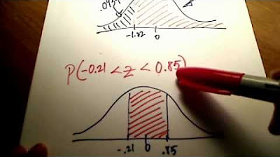
Use of a normal distribution graph to visualize the area between two z-scores.
Calculation of the probability of a car spending more than three minutes as 0.0655.
Discussion on whether it is unusual for a car to spend more than three minutes based on the calculated probability.
Comparison of calculated probabilities using different methods such as tables, StatCrunch, and calculator functions.
Highlighting the importance of accuracy in probability calculations and the slight discrepancies between methods.
Final conclusion on the normality of a car spending over three minutes in the drive-through based on probability thresholds.
Transcripts
Browse More Related Video
5.0 / 5 (0 votes)
Thanks for rating:

